DIMENSION REDUCTION AND SHRINKAGE (cont’d) STAT 627/427

Statistical Machine Learning, Baron

3. LASSO and RIDGE REGRESSION in package GLMNET

> library(glmnet)

# This package requires X-variables in a matrix

> X = model.matrix( medv ~ ., data=Boston )

> Y = medv

> ridgereg = glmnet(X, Y, alpha=0, lambda = seq(0,10,0.01))

# alpha is a “mixing parameter”. It combines Lasso and Ridge Regression. We only need the extreme values for now,

alpha=0 => ridge regression

alpha=1 => lasso

# So, which lambda is it best to choose? Run cross-validation…

> cv_ridge = cv.glmnet(X,medv,alpha=0,lambda=seq(0,10,0.01))

> names(cv_ridge)

[1] "lambda" "cvm" "cvsd" "cvup" "cvlo" "nzero" "name" "glmnet.fit"

[9] "lambda.min" "lambda.1se"

# For the selected values of lambda, we get

“cvm” = the mean cross-validation error

“cvsd” = its estimated standard error

“cvlo” = cvm – cvsd (lower curve)

“cvup”= cvm + cvsd (upper curve)

# All these can be plotted…

> plot(cv_ridge)

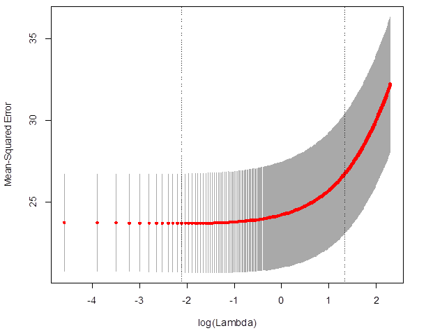
# Which lambda minimized the MSE?

> cv_ridge$lambda.min

[1] 0.12

> predict( ridgereg, cv_ridge$lambda.min, type="coefficients" )

(Intercept) 20.863586526

crim -0.068099108

zn 0.020536577

indus -0.068164404

chas 2.777651593

nox -5.514335229

rm 3.645249869

age -0.007642606

dis -0.532994082

rad 0.034679405

tax -0.002916331

ptratio -0.676296397

black 0.007674913

lstat -0.351786530

# Similarly with LASSO, only choose alpha=1

> lasso = glmnet(X, Y, alpha=1, lambda = seq(0,10,0.01))

# Compare the slopes estimated by ridge regression and by lasso

> plot(ridgereg)

> plot(lasso)

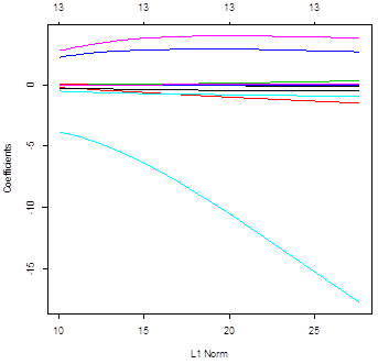
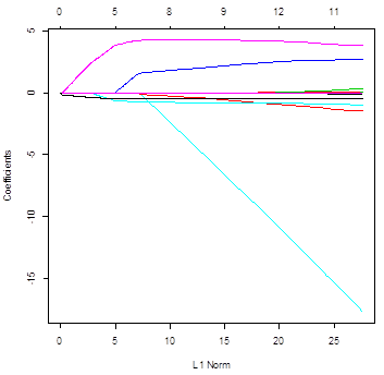
# Ridge regression uses all the variables – all slopes are not 0 for all lambda. Conversely, lasso does variable selection and sends some slopes to 0. The number of non-zero slopes is printed in the top.

> cv.lasso = cv.glmnet( X, medv, alpha=1, lambda=seq(0,10,0.01) )

> plot(cv.lasso)

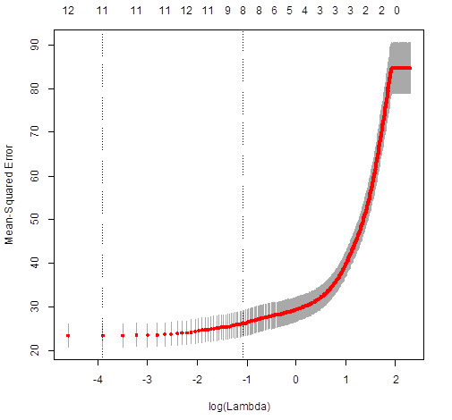
> cv.lasso$lambda.min

[1] 0.02

> predict( lasso,cv. lasso$lambda.min, type="coefficients" )

(Intercept) 18.739101467

crim -0.024356546

zn .

indus .

chas 2.009577446

nox -4.667589527

rm 4.273554725

age .

dis -0.401567952

rad .

tax .

ptratio -0.803881292

black 0.006716721

lstat -0.518576315

# For LASSO, the best lambda to use is 0.02. Some coefficients are 0 – these variables are removed from the model.

# Prediction for new values of X and cross-validation

> n = length(medv)

> Z = sample(n,n/2)

> lasso = glmnet( X[Z,], medv[Z], alpha=1, lambda=seq(0,10,0.01) )

> Yhat = predict( lasso, cv.lasso$lambda.min, newx=X[-Z,] )

> mean((Yhat - medv[-Z])^2)

[1] 23.62894

# This is the test MSE, estimated by the validation set approach.